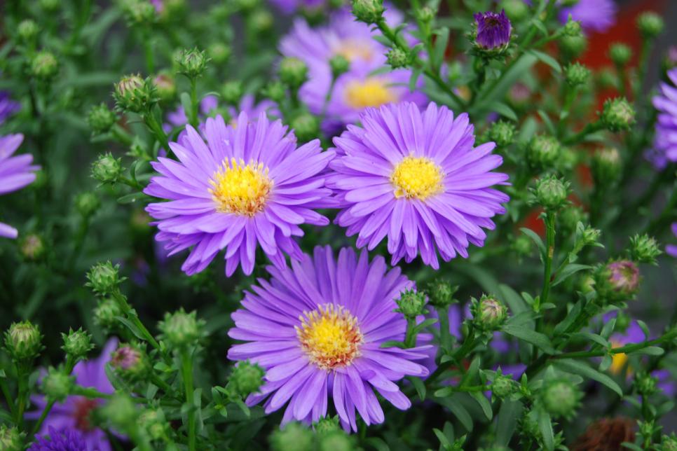
104 flower Image Classification


Download and then unzip the folder
In [ ]:
!unzip '/content/flowers_google.zip' -d '/content/flower/train/'
In [ ]:
!unzip '/content/test_flower.zip' -d '/content/flower/test/'
In [1]:
# !unzip 'source_location' -d 'destination_location'
Import fastai libraries and others
In [ ]:
from fastai.vision import *
from fastai import *
import pandas as pd
import numpy as np
import matplotlib.pyplot as plt
import seaborn as sns
Load the csv file it contains image ids and there corresponding labels
In [ ]:
df = pd.read_csv('/content/flowers_idx.csv')
label = pd.read_csv('/content/flowers_label.csv')
In [14]:
df.head()
Out[14]:
In [12]:
label.head()
Out[12]:
Locate a proxy path for the Deep learning model and the data
In [ ]:
path = Path('/content/flower/train/')  # Locates to the folder of train images
path1 = Path('/content/flower/test/')   # Locates to the folder of test images
forming DataBunch with test and train
In [ ]:
tfms = get_transforms(do_flip=True,max_rotate=0.1,max_lighting=0.15) # Each time it gets the image it will added some kind of transform like flip some times, rotate some times
In [ ]:
test = (ImageList.from_folder(path1,extensions='.jpeg')) # creating a test set
In [ ]:
data = (ImageList.from_df(df,path,folder='flowers_google',suffix='.jpeg',cols='id')
        # Creating a image list from dataframe  folder= folder_name, suffix = image_etxn, cols = column that contains image ids
                .split_by_rand_pct(0.15)
        # will take 15% of images as validation set
                .label_from_df(cols='flower_cls')
        # Label from dataframe cols= columns that contains category
                .transform(tfms)
        # add transforms
                .add_test(test)
        # add a test set
                .databunch(bs=128)
        # create a databuch for  the model
                .normalize(imagenet_stats))
        # normalize with imagenet stats because we are using a pretrained resnet model which was trained on image net
A look at the databuch formed
In [26]:
data.show_batch(rows=3) # rows = no. of rows
Total classes, length of train, validation and test set
In [36]:
len(data.classes),len(data.train_ds),len(data.valid_ds),len(data.test_ds)
Out[36]:
In [ ]:
fb = FBeta()
fb.average='macro'
Now here a learner is being created to train the model
In [39]:
learn = cnn_learner(data,models.resnet50,metrics=[accuracy,fb]).to_fp16() # .to_fp16() uses mixed precision traing computes operation in 16 bit floating point numbers
- Here I will use fast.ai lr_find() function to find a suitable learning rate
- Try to select a a bit before the minima
In [40]:
learn.lr_find()
learn.recorder.plot()
- Well the learning rate that corresponds to the minimum value is already a bit too high, since we are at the edge between improving and getting all over the place.
- We want to go one order of magnitude before, a value that's still aggressive so that we train quickly but still on the safe side from an explosion.
In [42]:
gc.collect()
Out[42]:
In [ ]:
lr = 1e-2
In [43]:
learn.fit_one_cycle(10,lr,moms=(0.8,0.7)) # training for 10 epochs
See in just 10 epochs we have reached a fbeta of 0.909 as well as accuracy of 91 %
In [ ]:
learn.save('model1') # let's save the model
learn.load('model1') # let's load it again and unfreeze it for further training
learn.unfreeze()
In [ ]:
#learn.export()
In [65]:
learn.lr_find() # let's use learning rate again to train some more
learn.recorder.plot()
In [68]:
gc.collect()
Out[68]:
In [69]:
learn.fit_one_cycle(3,1e-5,wd=0.2) # wd = weight decay it's regularization method to stop model from overfitting
In [ ]:
learn.save('model2')
learn.load('model2')
learn.unfreeze()
In [ ]:
#learn.to_fp32().export('/content/flower91.pkl')
In [ ]:
learn.to_fp32().export()
In [ ]:
#!cp '/content/flower91.pkl' '/content/drive/My Drive/Dataset'
In [72]:
learn.lr_find()
learn.recorder.plot()
In [79]:
gc.collect()
Out[79]:
In [83]:
learn.freeze_to(-2)
learn.fit_one_cycle(2,1e-6,wd=0.3)
Final Fbeta 0.91 as well as accuracy of 91.2 %
In [ ]:
learn32 = load_learner(path)
In [91]:
img = open_image('/content/flower/test/d9cb87ad0.jpeg')  # open the image using ope_image func from fast.ai
print(learn32.predict(img)[0]) # lets make some prediction
img
Out[91]:
In [ ]:
#!cp '/content/flower.pkl' '/content/drive/My Drive/Dataset/'
Let's interpret our model loses
In [92]:
interp = ClassificationInterpretation.from_learner(learn)
In [93]:
interp.plot_top_losses(12,figsize=(20,8))
In [96]:
interp.most_confused(min_val=3) # here it show max number of times it was confused between which clases
Out[96]:
In [98]:
pred,output=learn.get_preds(DatasetType.Test) # getting prediction of Test folder
we can export the model for production
In [ ]:
# using
learn.to_fp32().export('flower.pkl') # converting model back to 32 bit floating point numbers to save the model